9.2 Binding and Evaluation

Evaluation reduces a real expression to a single real, a composite expression to a simple composite with reduced components and a collection value to a simple collection with reduced items. When the evaluated expression contains variables, binding associates variables with definitions harvested from the workspace. Binding also deals with the complication of transient internal definitions within nested expressions. Binding takes place every time evaluation is performed; that is, when Evaluate is applied or when Plot displays a graph.

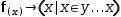
To begin with a simple example, consider the active expression x+1 and a companion definition x→2. One way to reduce the active expression to a value is to Substitute x and then Simplify . Because both operands are constants after substitution, simplification will produce a single value. Substitution as preparation for simplification becomes tedious as the number of variables increases, so sometimes evaluation is preferred.

Like substitution, Evaluate also examines the workspace for variable definitions. But instead of symbolic substitution, variables are bound directly to definitions, as shown in Figure 9.5. (For this purpose, suitable equations are promoted to definitions.) And, as opposed to the symbolic manipulation performed by simplification, evaluation performs numeric calculation directly on the bound values.

Bindings are ephemeral. They last only as long as necessary to complete evaluation. This is because expressions on the display are all independent; they can be added, deleted and manipulated symbolically in any order without concern for whether a variable has a valid definition. New bindings are established every time an expression is evaluated.

The process of binding begins with a set of unbound expressions and a set of definitions. The set of unbound expressions initially contains just the subject of evaluation. The set of definitions is created by examining each inactive expression for potential definitions. Binding then proceeds by examining each expression in the set of unbound expressions for variable names. If an association between a name and a definition can be made, the elaboration of that definition is added to the set of unbound expressions. Binding ends when all elements of the set of unbound expressions have been examined.

Since elaborations of definitions that are not referenced are never added to the unbound set and therefore never examined, a consequence of the binding process is that incompletely defined expressions that are never referenced are never bound. To illustrate, consider evaluation of x+1 in the presence of x→2 and y.→z-1. The latter expression cannot be bound because there is no definition for z (see Figure 9.6). But this does not matter when binding the first expression because no path of name to definition leads transitively from x to z.

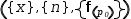
The description of binding uses the terms name, scope and namespace. A scope is a set of definitions; a namespace is a tuple of scopes. A definition is a name and its elaboration (essentially, just some expression). A name is a typed variable or a typed function name along with its formal parameter types. Both variable and function names can be sub- or super-scripted. A reference is a typed variable name or typed function along with parameter types taken from its arguments. A reference is resolved by searching the namespace and the scopes therein for the first occurrence of the name referenced. During resolution, references are bound to definitions.

The namespace created in the initial examination consists of a single scope called the global scope. When a definition's elaboration is considered at a later stage, it may contribute transient definitions to a new scope that augments the namespace.

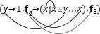
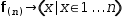
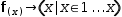
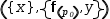
An example of this is a function that generates a tuple: fʈ(n)→(x|x∈1, n). To evaluate the expression fʈ(3), after examination the namespace consists of (, {fʈ(p_0)}). When the elaboration is considered, the namespace is augmented to include the parameter n in its own scope: ({n}, {fʈ(p_0)}). Before the tuple generator's template is considered, the upper limit n in the range generator is bound using the augmented namespace. Then x is added from the tuple generator to another augmentive scope yielding the namespace ({x}, {n}, {fʈ(p_0)}). The reference to x in the template is then bound. The result is shown in Figure 9.7.

In a slight variation on the same example, fʈ(x)→(x|x∈1, x) contains a confusion of x's. The x in the upper limit of the range is bound as before using the namespace ({x}, {fʈ(p_0)}) but because of nesting the x in the template is bound to a different definition using the namespace ({x}, {x}, {fʈ(p_0)}).

A more Byzantine example is given by fʈ(x)→(x|x∈y, x) (see Figure 9.8) . In the presence of y→1, the evaluation of fʈ(3) binds the lower and upper ranges using the namespace ({x}, {fʈ(p_0), y}). The upper limit is bound to the parameter and the lower limit is bound to a global name. Then, proceeding as before, the range control is added to its scope, the scope augments the namespace, and the template x is bound to the range control.

Binding also takes place within a serial tuple. A new scope is started when binding the tuple and variables defined within the scope remain local to the tuple. An example is shown in Figure 9.9.